Dynamics of Solar Convection

Jason Cooke and Kevin Wright

Introduction
Motivation
Optimization
Parallelization
Elliptic Equation
Results

First three sections: text and figures by Jason Cooke
Last three sections: original figures by Kevin Wright; text and revised figures by Dr. Steven R. Lantz

Introduction

Our main objective was to parallelize and optimize a program that simulated a particular model of solar convection. This required us to learn about methods of parallelization, methods of optimization, and to understand how and why the original program worked. The first two sections of this report talk about the model and how it was implemented in the original code. The third section deals with how the code was optimized, while the last three sections discuss how the code was parallelized.

The Fortran code used for the modeling was originally written by David Bryan, a participant in SPUR '94, under the guidance of Dr. Lantz. To take a look at his project, click here.

Motivation

Direct observations of the sun indicate much is happening in the convection zone. Most apparent are the granules, the tops of convection cells. One can also observe supergranules, which consist of a few hundred granules each. But it is unknown why the different types of cells come in distinct sizes.

By running simulations of different models, researchers can attempt to match their models to reality. Simulations also show how changes in parameters affect the behavior of the model. However, the more complicated the model becomes, the longer a program that simulates the model will take to run. Also, more complex programs tend to require more computer memory. These are both roadblocks to testing complex models.

Parallel computing offers an interesting solution to both problems posed above. By distributing the work load to many processors, the amount of time spent by each processor computing decreases. If the computer is a distributed memory machine, like the IBM SP2 at the Cornell Theory Center, the amount of data stored in each node can be reduced.

Because of the possibility of running simulations on data sets too large or time consuming for a single computer, we attempted to write a parallel program that would serve as a modifiable basis for running different models of the solar convection zone on a parallel machine. To test our code, we used a basic model that did not harness the full power of running a job in parallel.

Method

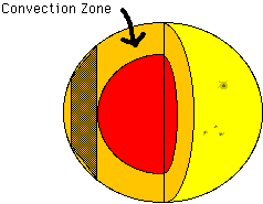
Pictured below is a cutaway of the sun showing the convection zone. This zone occupies the top 30% of the sun, where heat is transported from the hot inside of the sun to the cooler outside mainly by convection, instead of by radiative diffusion which is the case deeper inside the sun. The only part of the zone we are considering is the section represented by the shaded area. We assume this section is a good approximation to the actual shape of the convection zone in that area. We do not consider what happens in the zone at the poles.

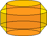
Below is the section of the convection zone we are considering, with the rest of the sun removed. A further approximation is imposed that there is only two-dimensional fluid motion, that is, no fluid moves parallel to the axis of the cylinder. This is a good approximation if the cylinder is rotating quickly enough about its axis (Busse and Or, JFM, 1986). Thus, the entire cylinder can be represented by one cross section.

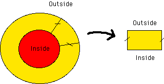
Another assumption is that all fields will be periodic along the disk. Then, the full disk can be represented by a section containing a single period. This section can then be approximated by a rectangle. It is on this rectangle that all the calculations are done in our simulation.

Disk with a hole in the center, section mapped to rectangle

Equations

The fields that we are concerned with are the temperature and velocity fields. For the Boussinesq convection model we are using, those are the only fields necessary. The equations below describe the restrictions on the fields and how the fields evolve and interact.

The Navier-Stokes Equation

$dv/dt + v\dot\nabla v = -1/\rho_0 \nabla p + \nu \nabla^2 v + \rho/\rho_0 g + 2 \Omega \cross v$

tells how a piece of fluid moves when there is a force acting on it; this is the basic equation of fluid flow.

The Heat Equation

$dT/dt + v\dot\nabla T = \kappa \nabla^2 T$

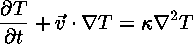
describes how heat flows into or out of a moving piece of fluid. Notice that this equation also involves the velocity.

The Incompressible Fluid Equation (Boussinesq Approximation)

$\nabla \dot v = 0$

says that the amount of fluid coming into a point is equal to the amount of fluid leaving that point.

The Equation Of State

$\rho/\rho_0 = - \alpha T/T_0$

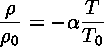
relates the density of a piece of fluid to the temperature of that piece of fluid. Notice that since the Navier-Stokes equation depends on the density, by this equation it also depends on the temperature.

Edge Conditions

Disk with a hole in the center, a section mapped to a rectangle

Since our equations are differential equations, we need to specify what the edge conditions are in order to solve them.

For the left and right edges of our rectangle, we require that the temperature and velocity fields must match on both sides. This is because the rectangle is a periodic section of the disk.

For the top and bottom edges, we require that the velocity of the fluid is parallel to the boundary. This keeps the fluid from flowing out of the top or bottom of the rectangle. For the temperature, we keep it fixed at the top and bottom corresponding to given outside and inside temperatures.

Derivative Approximations

Why Approximations Are Necessary

We approximate the fields by using arrays. The value in each box of the array is the value of the field in a corresponding area of the star. Let this area be called the control area. Any variation in the actual fields of a smaller scale than the control area is not seen in the array. Because of this, the control area needs to be selected so it is smaller than the size of the smallest important field variation.

The temporal components of our problem are also discrete. We have the equations set up to compute what the fields are at given time step intervals. As with the spatial approximation, variations in the fields that occur in a shorter time period than the time step are not observed. Therefore, the time step size needs to be selected carefully, as with the control area.

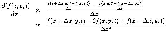
Because our fields are discrete, taking the derivatives poses a problem. Recalling from calculus, the derivative is defined by taking a limit:

$df/dx = lim_{h \rightarrow 0} (f(x+h) - f(x))/h$

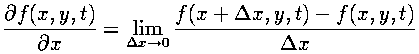
However, on a discrete grid there are no points arbitrarily close to each grid point, so the actual derivative cannot be calculated. Approximations to the actual derivatives can be computed using Taylor's Theorem.

Spatial Derivatives

We approximate spatial derivatives by using a symmetric finite difference approximation. For the first derivative,

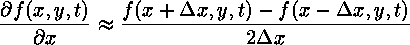
By applying Taylor's Theorem, this formula can be shown to be second-order accurate in the grid spacing. The second derivative is found by taking the derivative of the derivative. While asymmetric finite difference approximations are used for both derivatives, the result is symmetric.

d^2 f/dx^2 = (f(x+h) - 2f(x) + f(x-h)) / h^2

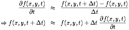
Temporal Derivative

In contrast to the spatial derivatives (where the field values on either side of the present point are used to calculate the derivative), we have the field value and time derivative at the current point and want to calculate what the field will be at the next time step. This amounts to performing an integration of the time derivative.

Because the Navier-Stokes and the heat equations can give the explicit time derivatives for the fields, provided that the values of the fields at the current time are known, this integration method could be used to advance the field through time. The asymmetrical derivative approximation used above (inside the second derivative) can be manipulated to give us an approximation to the time derivative integration:

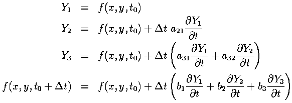
The above is a Runge-Kutta method, accurate only to first order by Taylor's Theorem. More accuracy is available from using a higher order method, at the cost of being more computationally expensive. By experimentation, we found that a third-order Runge-Kutta method was stable and accurate enough for our problem. Below are the general equations for a third-order Runge-Kutta:

In addition, the following relations between coefficients must be satisfied for the method to be third-order accurate:

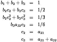
Notice that there are 8 variables and only 6 equations. This allows for classes of solutions to these equations.

Optimization

Since we are updating each part of the entire field at the same time, each one of the temporary variables used in the Runge-Kutta method above must be taken to be a temporary array, of the same size as our field array. This would require quite a bit of extra memory in our program.

Using a method that uses fewer working arrays could help to optimize our program for memory usage. Dr. Lantz proposed a method that uses only the field array plus just one working array. The structure of an algorithm that allows this is:

The extra equations that have to be satisfied for this to work, besides the 6 requirements mentioned previously, are the following:

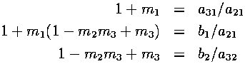
Using Maple, we solved the set of equations for the m's, a's, b's and c's after applying some extra conditions. Our extra conditions were to make as many coefficients as possible in the above Runge-Kutta algorithm equal to zero or one. When zero, no computation is required with the corresponding term. When one, no floating point multiplication is required. Each case could lead to increased program performance.

It turned out that some combinations gave valid solutions, while others did not. The results from solving the equations for are given here.

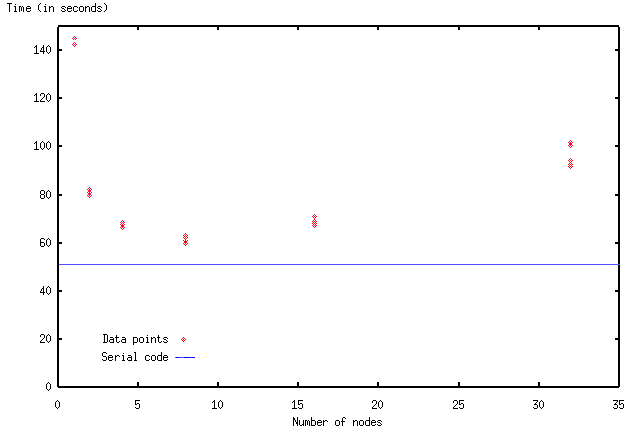
Parallelization

Domain Decomposition

A major goal of this project was to take the original program, now optimized to run on a single processor, and to parallelize it. The main thing to consider when parallelizing a program is how to divide the tasks over the processors. The most straightforward way to do it in this case is by domain decomposition, i.e. by assigning different chunks of the computational arrays to different processors. Each processor is then responsible for computing its own part of the simulated space. To be efficient, these computations should be kept as independent as possible.

But because of the various partial derivatives that must be computed, there is coupling between points on the grid. In most of the equations, derivatives are computed by finite difference formulas that depend only on neighboring points on the grid. So it seems that neighbors should be kept together as much as possible when assigning grid points to processors. However, there is also an elliptic equation (a Poisson equation) to be solved. When discretized, the Poisson equation becomes a large matrix equation, coupling together all the points along a row or column of the grid. This complicates the choices for how to divide up the grid among processors. We decided to cut our domain into horizontal strips, so that all data coupled horizontally would be present together on the same processor.

Interprocessor Communication Using MPI

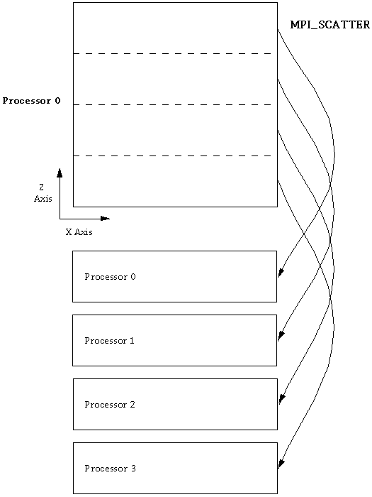
A parallel program requires extra software to allow communication between the independently running processors. For the parallel implementation of the code, we selected the MPI message passing interface to handle the interprocessor communication. The MPI standard includes many types of communication patterns, several of which are particularly well-suited to our application.

We set out to create a data-parallel program, in which processors are doing computations on different parts of the domain. So the first issue to address is: how should distinct strips of data be sent out to the different processors? It is very convenient to do this in MPI, because such strip initializations can be done with a single call to MPI_Scatter at the start of the job (figure). The inverse of this operation, MPI_Gather, is similarly useful for collecting data back to a single node. In our program, the gather operation occurs every time an output file is to be written; such output events occur at the end of a run and at regular intervals during the run.

Communication between processors must also occur at very frequent intervals during a run, in order to advance the code in time. There are two types of operations requiring communication. First, for computing derivatives in the time-evolution equations, data from neighboring points is needed; and it sometimes happens that these neighboring points reside on another processor, necessitating communication. Second, a communication pattern involving all the processors together is needed for solving the previously-mentioned global, elliptic equation. Parallelizing the elliptic solver is the tougher of the problems, so we will discuss it in detail in the next section. For the moment, we'll look only at the nearest-neighbor communications.

Communication of the Boundary Values

On each processor, a horizontal strip of data is surrounded by a border of extra grid points called "guard cells". The purpose of the guard cells is to handle boundary conditions (on exterior edges) or to serve as communication buffers (along interior partitions). The boundary conditions are periodic in the horizontal direction, so guard cells can be assigned locally, by wrapping around values from the opposite, matching side of the strip. On the vertical edges, guard cells are assigned in one of two ways. Where the edge corresponds to a physical boundary of the system, the physical boundary conditions are applied. But along an interior partition, updated information from a different processor must be brought in at regular intervals, in order to compute the derivatives in the usual way.

MPI provides a natural way for neighboring processors to communicate with each other, called MPI_Sendrecv. The sendrecv operation sends the data from a buffer in the local processor across to the designated processor, while at the same time receiving data from that processor (or another one) into a different buffer. With MPI_Sendrecv, data can be swapped between processors and received into guard cells, as we see in this figure:

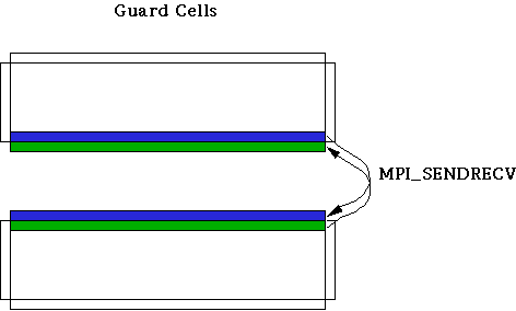
The operation needs to be done for each of the computational arrays. In practice, it is more efficient to pack a special buffer with all the necessary data from different arrays (temperature, vorticity, streamfunction) and do just one sendrecv operation (rather than two) in order to cut down on latency overhead--where latency is defined to be the cost to initiate a new message.

A special case arises when the strip has a physical boundary along one edge, because no communication is required. Instead, guard cell values are computed in the following way: imagine the physical boundary of the system to lie just beyond the last row of grid points. In particular, fix the location of the physical boundary to be exactly between the final row of data points and row of the guard cells next to it. Then, each guard cell value is defined such that the value halfway in between interpolates to the proper, physical boundary value. (The boundary condition on the temperature perturbation, e.g., is such that its value must be zero on the physical boundary.) The interpolating polynomial used for this procedure is second-order, so values from the last two rows of data, as well as the value at the physical boundary, are involved.

Elliptic Equation

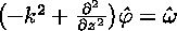
In our model, the time evolution of the 2D velocity field is not computed in the direct way from the Navier-Stokes equation. Rather, we manipulate our fluid equations mathematically so that we can deal instead with a quantity called the vorticity (omega), defined as the vector curl of the velocity. In 2D, the vorticity becomes a scalar, and it is therefore a more convenient quantity for computations than the two-component velocity vector.

An evolution equation for the vorticity can be derived by taking the curl of the Navier-Stokes equation. But the velocity is still needed in all the equations, so it somehow must be determined from the vorticity. This is done by exploiting the fact that velocity is divergenceless in the Boussinesq approximation. This implies that veolocity can be written as the curl of yet another field, called the streamfunction (phi). One can show that the vorticity and the streamfunction are related by

which is the Poisson equation. It is an elliptic partial differential equation to be solved for phi, given omega. This phi in turn determines the velocity: it is computed simply by taking derivatives (or finite differences) of the streamfunction, once it becomes known. Altogether, the computational procedure is as follows: first, the vorticity is explicitly advanced in time; then, the Poisson equation for phi is solved; then, velocities for the next time step are computed.

Computational Procedure for Solving the Poisson Equation

Clearly, the Poisson equation for the streamfunction must be solved every time the vorticity is updated. In effect, one must invert the Laplacian operator in the above equation. There are numerous ways to do this in an approximate fashion. In this section, we outline just one possibility, which is the one we actually implemented in the code.

The first step is to Fourier-transform the above equation in the x dimension. This is a natural enough thing to do, given the periodic boundary conditions that apply in this direction. The transformed equation is

where derivatives in x are simply replaced by multiples of ik. This equation can be discretized very readily. It is already discrete in k by virtue of the periodic boundary conditions, and the finite mesh spacing has determined the maximum k. In the z-direction, the remaining second derivative can be discretized using its finite-difference approximation. The overall result is

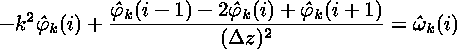
which can be rewritten as

Notice that the equations are completely independent in k but are coupled in the index i. This results in a set of independent matrix problems to be solved, one for each k:

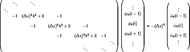The corners of the matrix have been neglected here; in general they contain special values that depend on the boundary conditions. The above matrix is a special, sparse type of matrix called tridiagonal, for which very fast algorithms exist (order N operations, to solve an N by N matrix). Unfortunately, these fast algorithms are inherently sequential!

Strategy for Parallelization

It might seem almost pointless to try to parallelize the above scheme. Probably it would be, were it not for two additional facts:

we have a large number of these matrices to solve all at once (one for each k); and
the problems are all completely independent of one another.

This mutual independence admits the possibility of a parallel solution. Dr. Lantz suggested the following procedure (where the leading "//" symbol marks operations that can be done in parallel):

// Take Fast Fourier Transforms (FFT's) of the vorticity in the x-direction. (Remember, the data all start out in horizontal strips.)
Transpose the transformed vorticity data across processors so that each processor now has all the i's for just a subset of the k's.
// Solve the independent tridiagonal matrix equations--one for each k--by using the best available serial algorithm locally.
Transpose the streamfunction data back across processors, so that each processor has all the k's for just a subset of the i's (same as initially).
// Take inverse FFT's to determine the streamfunction.

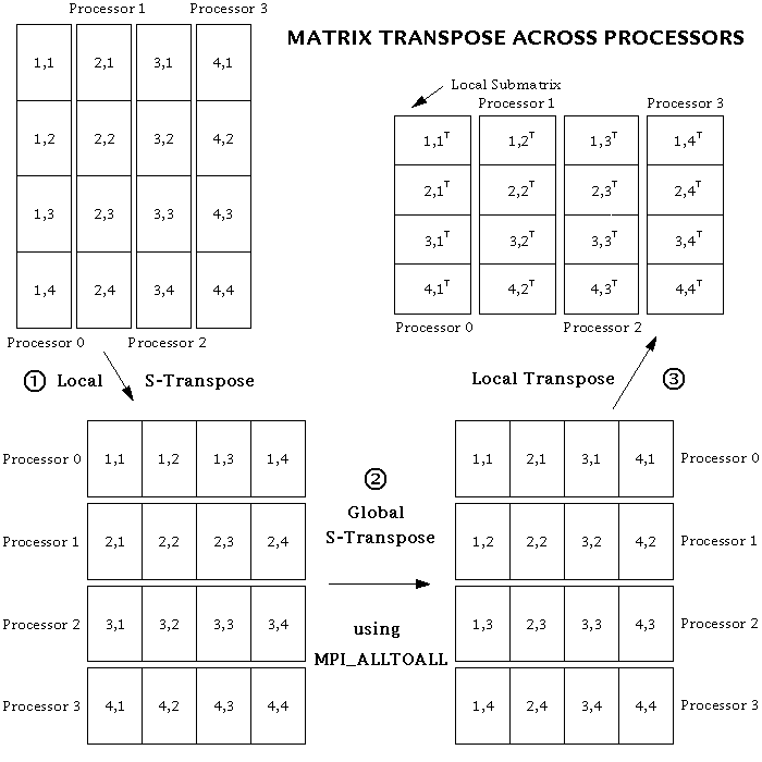
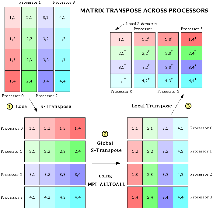
It seemed at first that the specified data movements could be done very simply by using the MPI_Alltoall subroutine. In MPI_Alltoall, each processor sends a message to, and receives a messages from, all the other processors. In our case, this message should simply consist of a submatrix of the original matrix. But it turns out that there are additional, local transposes that need to be done on the submatrices in order to get the data into the correct places, both before and after the MPI_Alltoall operation. This is because MPI_Alltoall does not transpose any of the data within a submatrix; it merely transposes submatrices intact. Furthermore, MPI_Alltoall only works when each submatrix has its elements stored in contiguous memory locations. So, in place of the simple call to MPI_Alltoall (in steps 2 and 4 above), the following three-step procedure has to be performed:

// Reorder the data so that the local column vector of submatrices becomes a row vector (assuming the data are ordered in memory in the standard Fortran or "column major" style). This operation can be called an "s-transpose", an abbreviation for either "submatrix transpose" or "stick transpose", because sticks of data are being moved around in memory.
Using MPI_Alltoall, do a global s-transpose of the submatrices across processors. Each processor now has all the i's for just a subset of the k's. But the data are still ordered so that the k's are counted first.
// Perform a normal matrix transpose on the entire matrix defined by the row vector of submatrices (i.e., on the whole local piece of the distributed matrix), in order to have the i's counted first.

The global matrix transpose scheme can best be explained by a picture. (Dr. Lantz has also created a color version.) Note that the transpose procedure works equally well if the order of the steps is reversed.

Results

After parallelizing the code, it was time to try out some simulation runs to see if it was working properly. In particular, we wanted to create visualizations of the simulation results. The tool we used to help us visualize our data was IBM's Data Explorer. DX allowed us to render a sequence of images, representing the fluid variables at fixed moments in time. These frames could then could be concatenated into an animation. Here is an MPEG movie showing a typical thermal Rossby wave, starting off from a stationary state (plus some "noise") and then settling into steady traveling motion. Contours of the streamfunction, shown as black lines, represent streamlines of the flow, while the color shading corresponds to the fluctuating part of the perturbed temperature (i.e., what's left of the temperature perturbation after a purely conductive profile has been subtracted off).

Overall, we succeeded in meeting the main goals of this project, which were:

To parallelize Dr. Lantz's code for simulating thermal convection in a rotating frame of reference, and
To improve its serial performance through more efficient Runge-Kutta time stepping.

The final results of our efforts were somewhat mixed, however. Some modifications worked well, while others did not.

Trials of several tableaux from the new family of Runge-Kutta schemes showed that they all ran stably and well, proving to be about 10% faster than the original code.
A working parallel version of the code was assembled, and tests with it were successful, in that they generated physically correct results. This was proved by setting the code's parameters to correspond to a regime where solutions to the fluid equations are expected to be stable thermal Rossby waves (Busse and Or, JFM, 1986). A plot of angular frequency vs. the rotation parameter (eta) shows excellent agreement between the results of our simulations and the theoretically predicted values for the phase speed of this type of traveling wave.
Unfortunately, a plot of execution time vs. number of processors shows that the parallel version of the code did not produce a speedup for any number of processors. In other words, the original, single-node version always ran faster than the parallel version.

The main unsolved problem from this project is how to improve the poor performance of the parallel code. Performance problems like this one can be diagnosed by tracing execution of the program on all the processors, then merging individual traces together and visualizing them with a tool like "nupshot". The tracefile visualization from our code shows that the main culprit is the Poisson solver routine, which is what was expected, because this routine involves the most coupling between grid points. It is obvious from the tracefile that far too much time is being spent in MPI_Alltoall calls. Basically, too little computation is occurring between these communication events; each MPI_Alltoall takes a relatively long time to complete due to the finite speed of the high-performance switch. Thus, there is a fundamental problem with this method on the SP2 architecture, because unproductive communication tends to dominate. We believe that the only remedy for this problem is to find a new parallel algorithm that does not require so much communication.

Back to Cover Page