Justin Boland, July 30, 1997
![]()
When a fluid is in equilibrium, the most dense fluid has settled on the bottom and the least dense fluid has been forced to the top. Applying a temperature gradient by heating the bottom fluid will cause the fluid at the bottom to gain energy and become less dense. A bit of it may begin to rise, expanding in response to the lower pressure as it goes. This packet may then find that it is still less dense than the fluid at its new level, so it continues to rise. When the packet of fluid gets to the top it gives off its energy and becomes more dense. Eventually, it sinks to the bottom and becomes heated again. The cycle will continue to repeat itself as long as the unstable temperature gradient exists. These actions are called convection.
Fusion and fission occurring at the center of the sun release a tremendous amount of energy which is radiated outward in all directions. This energy transfers itself from the center to the outside of the sun in the forms of radiation, conduction, and convection. Radiation dominates over the others until a depth from the surface of 200,000 km (about 30 percent of the solar radius) is reached; from there to the surface, convection dominates. Supergranulation is one form of convection where large flows of plasma circulate from deep in the sun toward the outer layers. Cooler, more dense species from above displace the hotter species forcing them to rise at a speed about 10 m/s. Near the surface, the lighter species radiate their energy and become heavier. Supergranulation typically occurs on the scale of 30,000 km horizontally and between the depths of 8000 and 10000 kilometers and at a temperature gradient ranging from about 6000 degrees Kelvin to a few million degrees Kelvin. Due to the extreme depth of the convection, density gradients also play an important factor in fluid flow in contrast to the laboratory model of convection. These granules are called "super" because they are about 30,000km in diameter where other solar granules near the sun's surface are only a few hundred kilometers in diameter. When the gas reaches its final height, it moves horizontally before receding. Horizontal speeds average around 500 m/s which is about 1100 mph! The typical life span of a supergranule is about half a day and the gas flow achieves about one cycle before the supergranule cell loses shape. Therefore, we are dealing with non-stationary convection patterns in the sun.
![]() Diagram
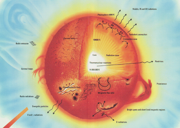
of the Sun, Courtesy (NASA/ESA)
Diagram
of the Sun, Courtesy (NASA/ESA)
![]()
![]()
![]()
Modeling the flow of gas and plasma in the sun was accomplished through magnetohydrodynamic (MHD) equations. The equations used in our simulation model a two dimensional system with four second order partial differential equations. The equations describe the laws for the evolution of momentum(two equations), magnetic field, and entropy in the system.
Last year's SPUR report gives a more detailed explanation of a related model that uses these equations. Our model is based on the anelastic approximation rather than the Boussinesq approximation, so the heat equation and equation of state are more complex than previously.
![]()
![]()
![]()
The MHD equations were linearized, i.e. the nonlinear terms were removed, a valid thing to do for small-amplitude perturbations. Dr. Lantz worked together with Dr. Yuhong Fan to produce the final set of equations that we used in this project.
![]()
![]()
![]()
Numerical Recipes in C describes this method as:
"The differential equations are replaced by finite difference equations on a mesh of points that cover the range of integration. A trial solution consists of values for the dependent variables at each mesh point, not satisfying the desired finite difference equations, nor necessarily even satisfying the required boundary conditions. The iteration, now called the relaxation, consists of adjusting all the values on the mesh so as to bring them into successively closer agreement with the finite difference equations and, simultaneously, with the boundary conditions." (page 599)
We replaced the four second-order derivatives with four equations for first-order derivatives. This yielded a system of eight first-order differential equations and an implied ninth equation that represented the eigenvalue for the growth rate of the fluid. To mutate these equations into finite difference equations, all derivatives had to be replaced with their discrete, finite-difference representations.
Each of these equations had to be derived to obtain the coupled, nonlinear set of algebraic equations to enter into the code.
![]()
![]()
![]()
![]()
As it solves the system of equations, the 9eqns program generates an output file for each iteration. The program continues to improve the approximation to the solution until the error between the value of the current approximation and the previous one is less than 10-6.Each of the data files output from the 9eqns program holds data that can be used to plot all 9 functions for the current iteration. Each plot is important in that it can graphically detail the solution for the variable in the current step in the process of solving the system of equations. However, when all the frames for any one of the variables are viewed in chronological succession, there is a deeper meaning that can be appreciated. These graphs can be turned into animations for each variable with as many frames as there are steps in solving the system. From these animations, it can be easily seen how the algorithm alters the eigenfunctions and the eigenvalue to match the equations. To this end, we developed code that would run the 9eqns executable, graph each variable for each frame, and then create an mpeg animation of each variable for all frames.
We worked on an AIX platform with perl scripting capabilities. Perl was chosen because many of the commands are similar to C and because perl is well integrated with the standard input/output from the AIX system.
![]()
![]()
![]()
![]()
After a few fixes to the code, the resulting eigenvalue received from the program nearly matched the expected value for the simplest scenario. In this scenario, we used a initial guess with no nodes (normalized wavenumber = 1) and an initial guess for the eigenvalue. The animation shows that, although the eigenvalue started near its final value, the values for the other functions needed some adjusting to solve the system. It is interesting that the animations show how the initial guess for the variables transforms into the expected functions. Initially, the functions were all given as being regular sinusoidal functions with only a scaling factor. Notice that as these function evolve toward the solution, they remain somewhat sinusoidal but become weighted.
As a next step, the perl script was modified to run the 9eqns executable in separate directories, each corresponding to a different wavenumber based on the input initial guesses for the eigenvalue and eigenfunctions. An expected result of the code is that the highest eigenvalue obtained was the same eigenvalue that resulted from the simple scenario. All other eigenvalues obtained were negative. This finding is significant because only positive eigenvalues result in exponential fluid growth whereas all negative eigenvalues represent a system where the motion of the fluid is exponentially damped. One can reason from this that certain conditions must exist for the convection cycle to occur, namely that the heat dissipation must not be faster than the motion of the fluid. As discussed earlier, a negative entropy gradient (in z) is required to force the fluid to move.
The development of the perl scripts to automate the processes involved will hopefully save hours of monotonous typing. The last run of the script generated 70 different runs of the code with wave numbers ranging from 1 to 70. All output from the 9eqns program was turned into mpegs. This process took approximately 1 day and thirteen hours running continuously on one node of the IBM SP2 supercomputer. This would have taken a significantly longer time if all commands had to entered by hand.
![]()
![]()
![]()
![]()
Much thanks to Steve Lantz for being the best advisor.
Thanks to Bob, Kathy, and the rest of the theory center for making my experience
at Cornell one of the best times of my life.
Thanks to Jennifer Jones for informing me that SPUR exists.
And thanks to all my new SPUR friends for being so much fun.
I'm going to miss all of you.
This work was conducted using resources of the Cornell Theory Center (CTC). CTC receives major funding from the National Science Foundation and New York State, with additional funding from the National Center for Research Resources at NIH, the Advanced Research Projects Agency, IBM, and other members of CTC's Corporate Research Institute.
![]()
![]()
![]()
![]()
difeq.c is the module that I wrote to solve the system of equations for the growth rate given an initial perturbation.
everything is the perl script that I wrote to run the 9eqns executable with command line arguments to control a variable number of subdirectories representing each wave number, a starting and stopping variable number, and the initial guess for the eigenvalue.
Numerical Recipes in C by Press, Flannery, Teukolsky, Vetterling
Cambridge, UK University Press, 1988
Tritton,D.J. Physical Fluid Dynamics,Van Nostrand Reinhold Company Ltd. New York, N.Y. 1977
Seab, C. Gregory. Astronomy, Springhouse Corporation. Springhouse, PA 1995
Giovanelli, Ronald. Secrets of the Sun, Cambridge University Press, Cambridge, UK 1984
Lantz, Steven R. "Magnetoconvection Dynamics in a Stratified Layer. I. Two-Dimensional Simulations and Visualization"The Astrophysical Journal, March 10 1995
Lantz, Steven R. "Magnetoconvection Dynamics in a Stratified Layer. II. A Low-Order Model of The Tilting Instability,"The Astrophysical Journal, March 10 1995
http://hao.ucar.edu/public/research/mlso/mlso_homepage.html
http://umbra.nascom.nasa.gov/images/latest.html
http://orpheus.nascom.nasa.gov/synoptic/
http://pore1.space.lockheed.com/SXT/homepage.html
http://www.acim.usl.edu/SOLAR/sun/sun_views.html
http://bang.lanl.gov/solarsys/sun.htm
![]()
![]()
![]()
