Convection is the result of an instability. It occurs when a bubble of gas at a certain depth gains more heat energy than the surrounding gas. This increase in heat energy causes the bubble to expand and become less dense than its environment. The bubble then feels a net buoyant force upward, so it begins to rise. After a while, the bubble will lose its heat to its surroundings, contract, and become more dense. Therefore, it is forced downward by the buoyant force, where it will again become heated and continue the cycle. However, the convective process inside the sun is not this simple. There is a difference in density of more than an order of magnitude from the bottom to the top of the convection zone. For this reason and others, convection is more turbulent inside the Sun than it is in the Earth's atmosphere or in laboratory experiments.
The reason it is known there is a convection zone inside the Sun, comes from observations of the Solar surface. In white light, a granulation pattern appears on the Sun's surface due to the smallest convection cells which have diameters on the order of a few hundred kilometers.
The x-ray image of the Sun to the left shows the supergranulation pattern. Each supergranule is composed of many smaller granules. Supergranules typically have a horizontal diameter of 30,000 km and extend to depths of 8,000 - 10,000 km. Strong magnetic fields are trapped in the the downflow regions of supergranules; therefore, in the image the brighter areas are sinking and the darker areas are rising.
Understanding the workings of the convection zone is important, because the magnetic irregularities that convection produces, such as sunspots, can affect the climate of the Earth. However, it is not possible to recreate the interior of the Sun in a controlled setting because of the enormous temperatures and density differences involved. Therefore, the only realistic way to learn more about the Sun's interior is through numerical modeling.
Dr. Lantz has developed a number of models in the past that have been concerned with the workings of the convection zone. However, these models have assumed that the Sun is composed of an ideal gas, but this is not true. For the present model, Dr. Lantz is building upon a previous model known as the anelastic magnetohydrodynamic equations. This time around though, the goal is to add depth dependencies to the thermodynamic variables that account for things, such as ionization, which are not associated with ideal gases. The end result will hopefully be a better understanding of the convection zone.

The term anelastic refers to the fluid properties of the gases that are being studied. An anelastic model can be thought of as being a happy medium between modeling a fully compressible and an incompressible fluid. A model of a fully compressible fluid would be most like that of the interior of the Sun because it could account for the great density differences in the convection zone. However, this model becomes more complicated to solve because of the many terms involved. An incompressible, or Boussinesq, fluid is much easier to model, but it is not a realistic representation of the Sun. A compromise is the anelastic model, which is built around a background that allows variables like density to vary with depth. This results in easier computations than the compressible model, but better results than the Boussinesq.
The other term describing the model, magnetohydrodynamic, refers to the forces acting on the fluid. This model involves magnetic fields along with buoyancy forces that drive the convection inside the sun.
The widely used mixing length theory of convection (MLT) gives a description of how heat is transported in stars. The basis of this theory is that a small velocity and a large scale of convection are sufficient to transport large quantities of heat. Perturbations are added to a background state that is hydrostatic and isentropic; that is, the buoyancy force is balanced by the force resulting from the local pressure gradient in the vertical and there are only infinitesimal perturbations to entropy resulting from compression and expansion during vertical motion. Convective motion results from these perturbations. One main problem with MLT is that it deals with large scales, but convection also occurs on smaller, turbulent scales. Specifically, Dr. Lantz is concerned with the treatment of the diffusion constant which determines the background entropy. MLT uses a diffusion constant that takes place on large scales, but in his paper, Dr. Lantz used a constant that works on a turbulent space scale. The objective now is to use both constants with this set of equations and then determine which constant is more suitable for the model. The following are conditions for a hydrostatic and isentropic state:
The next step in the development of the model is to write out all the governing equations: the momentum, entropy, and continuity equations, Ohm's Law, the equation of state, and the first law of thermodynamics. Then the equations are scaled. First, the variables are rewritten as a product of a reference value of the variable and a new value of the variable (i.e., x = xx*, where x is the reference value and x* is the new value of the variable. This is done to make the values of the variables smaller, so that it is easier for the computer to deal with them in computations. Then, the background isentropic and hydrostatic state is taken to be the lowest order state. Next the equations are non-dimensionalized by dividing through each equation by the coefficient reference values of the dominant term in the equation. For example in the momentum equation, all the terms are divided by the product of the reference values of gravity and density, which is the coefficient of the buoyancy term. In the case of the momentum equation this results in two terms that are around a value of 1 ( the pressure gradient and buoyancy terms ), and the remaining terms which are of a value which is much smaller than 1. After completing this process the equations appear as the following:
Note: Variables subscripted with a 0 have only a depth dependence, whereas, those subscripted with a 1 have a dependence on both spatial dimensions and time. Epsilon is a number << 1. The Reynolds number is a dimensionless value of the ratio of inertial to viscous forces, and the Peclet number is the product of the Reynolds number and the ratio of the dissipation of momentum to heat.
To further simplify the equations, Dr. Lantz has gone through a series of steps that reduces the number of time dependent thermodynamic variables to one. This can be done because the changes in entropy, temperature, and density are linearly related. In this model the entropy remains as the only quantity that has a time dependence. Furthermore the continuity equation and the initial condition of Ohm's Law place restrictions on both the velocity and the magnetic field. They become dependent on vector potentials or (in 2D) stream functions. This results in the following set of four second order partial differential equations.
Previously, a code was developed which solves for the dependent variables in the case of an ideal gas. Therefore, the background variables could be computed computed based on the depth and value of a single parameter known as the polytropic index. To update the code, this dependence has been removed and the values of the thermodynamic variables were changed to take into account the partial ionization of the gases that happens inside the convection zone.
By plugging in these exponential functions of x and t, the derivatives with respect to x and t become the product of the original exponential function and a constant in x and t. Every term in the equations contains an exponential function, so they all cancel. Therefore, the dependence on x and t is removed from the equations. The result is a set of four ordinary differential equation where z is the only independent variable. The four second order equations are then converted into eight first order equations. A ninth equation is also obtained by setting one function equal to b, the eigenvalue of the resulting matrix equation.
The above nonlinear ODE's are linearized to form a matrix equation of the form Ay = 0 where A is a matrix of coefficients, and y is a vector containing values of the dependent variables, at different depths, z. To solve this equation, a former research assistant, Justin Boland, put together some Numerical Recipes that use a relaxation method. First, a one dimensional grid of points is created, then an initial guess is input to the code for values of the dependent variables at each of the mesh points on the grid. The code then solves for corrections to the initial guess and adds these corrections to the guess until a certain error tolerance is reached. The numerical approximation is said to "relax" to the actual solution.
The eigenvalue that is obtained from the linear stability code is important, since it represents the exponential rate of growth of the dependent variables. These exponentially growing functions start out as the perturbations to the background state mentioned above that drive the convection. Therefore, if the resulting eigenvalue is negative, then the perturbation becomes small as time progresses. Conversely, if the eigenvalue is positive, then the perturbation along with the convection will grow with time. Also, the final values from the approximation can be multiplied by sinusoidal functions of x to obtain initial conditions for the simulation.
As with the original code that solved the set of 2-D time dependent equations, Justin Boland's code also assumed that the gas is ideal. Therefore, the code has been altered so that the thermodynamic values with respect to depth now account for partial ionization of the gases involved.
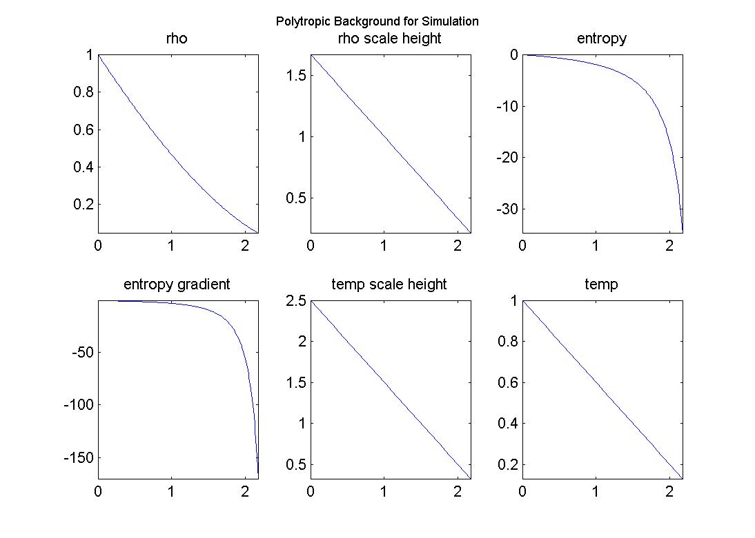
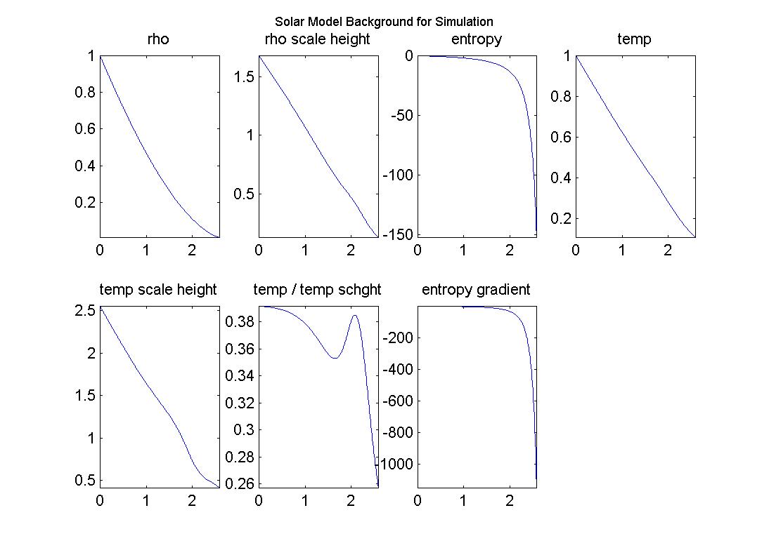
The first two plots are for backgrounds in which the dynamic viscosity is constant, and the last two plots are for backgrounds that allow the dynamic viscosity to vary with depth.
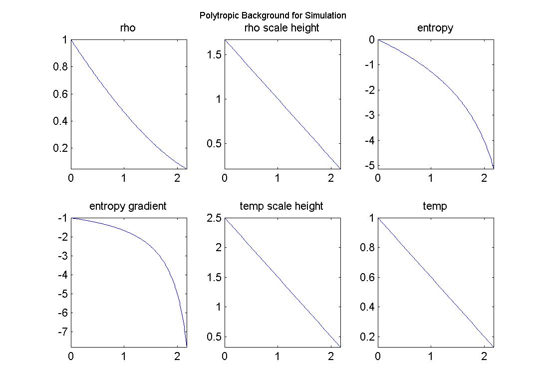 Polytropic Background, mu = constant
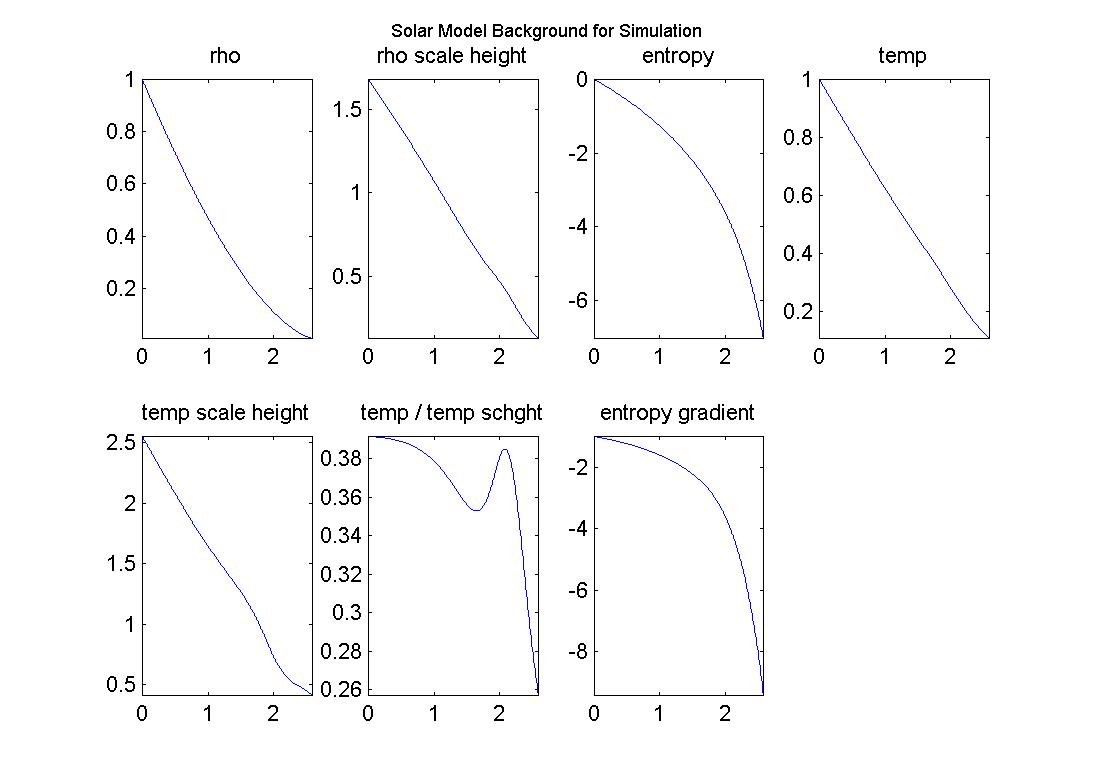 Solar
Model Background, mu = constant
Solar
Model Background, mu = constant
 Polytropic
Background, mu = rho
Polytropic
Background, mu = rho
 Solar
Model Background, mu = rho
Solar
Model Background, mu = rho
 Linear
Stability Code Animation (Polytropic Background)
Linear
Stability Code Animation (Polytropic Background)
 Simulation
Animation (Ionizing Gas - Settling to a steady state)
Simulation
Animation (Ionizing Gas - Settling to a steady state)
For the following runs the value of mu and kappa was held constant and equal to 1.
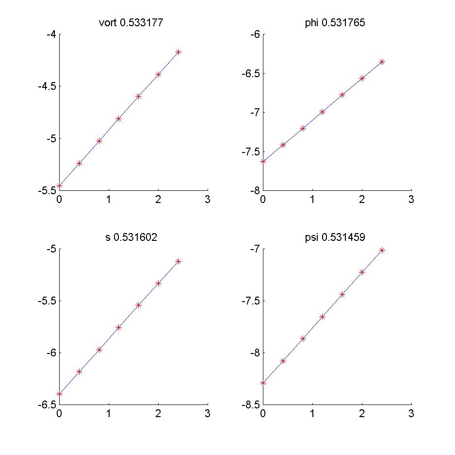
Given a polytropic background and the parameters (in dimensionless units):
Note: The previous eigensolver had a nonlinear term in the calculation of entropy which produced a growth rate of 0.557 given the same parameters above. By coincidence, the simulation gave a growth rate of 0.555.
Linear
Stability Code Polytropic Background
Growth Rates From Simulation
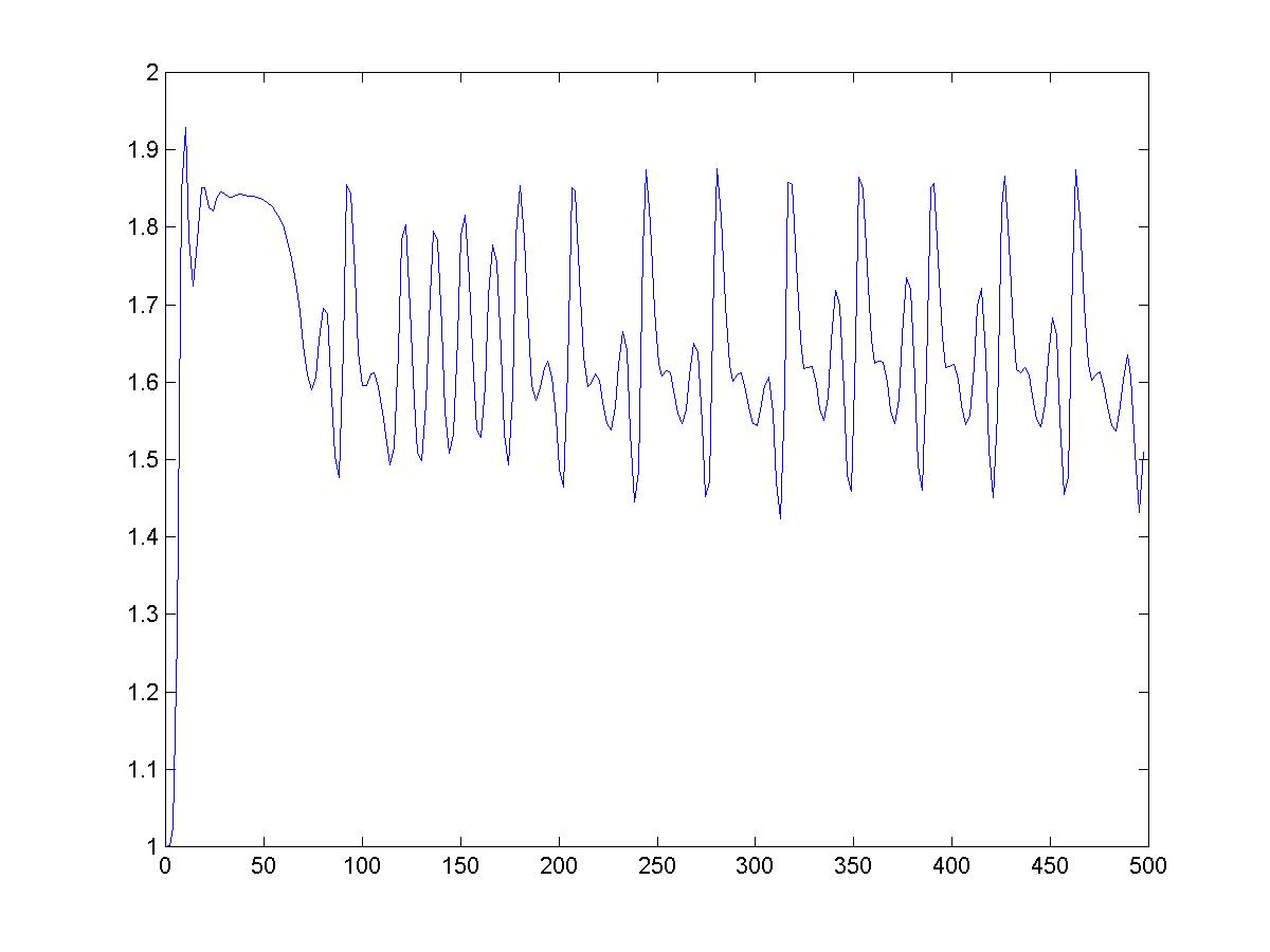
The simulation was also tested for long-time development in the nonlinear regime. Below is a plot of the Nusselt number, which is the ratio of the total heat flux (convective and diffusive) to the diffusive heat flux. The simulation was run on a 64 x 64 grid with a 180 G magnetic field imposed at the lower boundary. The plot matches well with figure 3b from Dr. Lantz's paper.
Nusselt Number Ratio of Heat Fluxes
Simulation
Polytropic Background
re = 200 All values settle to a steady state.
re = 800 The value fields begin to oscillate before t=200.
re = 1600 Oscillation is more erratic. In the plot of vorticity, notice
the jet-like structure that develops in the upflow.
re = 2400 Final state of previous run was used as input to this run.
The erratic "firehose" oscillation continues.
(polytropic background) re = 2400 This is the same as the last run
except that a polytropic background was used. The goal was to see if the
oscillating behavior was the result of partial ionization. The contour
intervals were changed so that there are more contours at smaller values.
However, the coloring scheme was not changed (Note: Z = 2.35 for this run.)
(phase shift) re = 2400 Again, the Reynolds number is 2400 and the background is based on the
Solar Model. The initial
fields came from the linear stability code, and they were shifted by pi/2,
to better see what was happening in vorticity at the boundaries.
(continuation) re = 2400 A continuation of the run of with re = 2400, and a Solar Model Background.
re
= 800 Oscillation occurs.
In the following runs the value of mu and kappa were allowed to vary with depth and are equal to the value of rho.
While trying to incorporate a depth dependent dynamic viscosity into the two codes a number of bugs were found. After running the updated codes with a constant dynamic viscosity, the eigenvalue and growth rates were found to match to three decimal places.
However, with mu and kappa allowed to vary, the eigenvalues and growth rates differed by greater than 15% for low values of the Reynolds number (re = 4), while the two parameters would match to two decimal places when higher values of the Reynolds number (re = 40) were used.
The grid size was then increased from 128x64 to 256x128, and the growth rates were found to match to three decimal places for all values of the Reynolds number. The following table summarizes the results.
Table Comparing EigenValues and Growth Rates Note: A polytropic background was used for these runs, and the values of the parameters are the same as values used for the polytrope tests above, except for the values of re and rm which are specified in the table.
For the following runs, a 256x128 grid was used
Parameters:
re and rm = 40 Polytropic Background. The fields settle to a steady state.
re and rm = 110 Polytropic Background. A travelling wave develops and the downflows tilt slightly toward
the end.
re and rm = 110 Solar Model Background. The fields oscillate slightly.
The smaller structures that would indicate supergranulation have not been observed yet in any of the simulation runs. The new round of tests with a varying viscosity have just begun, so it is still unclear what will result from these runs. However, early results of these runs show that the difference in the way the dynamic viscosity is treated may be just as interesting as the differences that result from changes in the background due to partial ionization are.
More driving in the form of higher Reynolds numbers will most likely be needed to observe the desired structures. Therefore, further tests will involve larger grid sizes which will result in more calculation time.
Numerical Analysis by Burden, Faires, Reynolds
Boston, MA, Prindle, Weber & Schmidt, 1981
Numerical Recipes in C by Press, Flannery, Teukolsky, Vetterling
Cambridge, UK University Press, 1988
The Matlab 5 Handbook by Redfern, Campbell
New York, Springer, 1998
Ammeraal, Leendert. C For Programmers, John Wiley & Sons, New York, 1986
Giovanelli, Ronald. Secrets of the Sun, Cambridge University Press, Cambridge, UK 1984
Lantz, Steven R & Fan, Yuhong. "Anelastic Magnetohydrodynamic Equations For Modeling Solar And Stellar Convection Zones," The Astrophysical Journal Supplement, March 1999
http://www.tc.cornell.edu/~slantz/SPUR/SPUR97/Justin
http://www.tc.cornell.edu/~slantz/SPUR/SPUR96/Cynthia/report.html
http://umbra.gsfc.nasa.gov/images/lastest.html